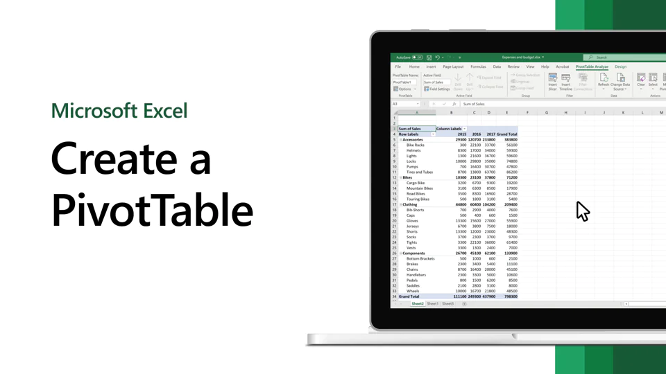
How To Create A Pivot Table In Excel Spreadsheet?
In this episode of friendly learning, we are focusing, on Microsoft Excel’s powerful features notably the pivot table. A pivot table helps you to summarize larger sets of data efficiently. Usually termed complex, in this blog, we will show you how to create a pivot table in Excel in a few easy steps to believe. Before diving into the depth, let us have a sneak peek into the general understanding of the feature and why it is necessary to use a pivot table.
What is a Pivot Table?
Generally, a pivot table is the overall summary of your data practically, it information is packaged in a chart which makes it easier to work, explore and report onwards. These tables are most useful when working on larger datasets that include long rows or columns to keep good track of data and doing one on one data comparisons. The ‘Pivot’ part of this feature originates from the fact that data can be viewed from different perspectives like a pivot. The basic function of this incredibly organized table is to make data recognition easy and useful.
What are Pivot Tables used for?
Here are five instances where you can make great use of a pivot table:
1. Comparing sales totals of different products.
Suppose you have a worksheet that contains your product monthly sales data in the form of — product 1, product 2, and product 3 — to figure out which of the three sets has been the customer’s favourite choice you will need to look into the worksheet. Manually speaking, you will need to do the whole process one by one. Now suppose your sales sheet has thousands of rows; in this case, you are certainly not getting any weekend breaks on your part. Here is where the pivot table fits in; you can automatically arrange the whole sales sheet for products 1, 2, and 3 and calculate their sums in less than one minute.
2. Showing product sales as percentages of total sales.
Pivot tables naturally showcase the total number of each column and row as soon as they are created. But this is not the only mathematical trick that you can perform with Pivot tables. These tables allow you to enter quarterly sales data for 3 different products into an Excel sheet. The total sum is automatically generated at the end of every column. But the story does not end here folks you can also calculate the percentage “%” of these product sales which has contributed to overall company sales. To calculate the percentage of the total product sales you simply have to click the cell carrying sales total sum and select ‘Show Values As >% of Grand Total’.
3. Combining duplicate data.
In this hypothetical situation, you have created your blog redesigning and happened to be left with updating a few URLs. Unfortunately, your software ended up splitting the ‘view’ metrics for a single post between two URLs. Now to get your hands on accurate data you will have to merge these duplicates. This is the reason why Pivot Table is used to instantly combine all the metrics from the duplicates. You get to summarize your data effortlessly using Pivot Table.
4. Getting an employee headcount for separate departments.
Pivot tables are really helpful in creating accurate calculations of data that are otherwise not present in Excel tables. However, the main thing which is present is the counting of rows in almost every table. Creating and managing a Pivot Table is remarkably simple once you become familiar with the process. For instance, if you have a list of employees in your Excel sheet, right next to them you have their domains/departments names in which they serve, then you can create a Pivot Table from this much information which shows every department name and number of employees serving in those departments. Using a Pivot Table reduces manual sorting of Excel sheet and make business internal operations faster.
5. Adding default values to empty cells
It is a myth that every dataset that you enter in your Excel sheet will populate all the cells within that sheet. If you are looking for new data to update your Excel then you might get confused by looking at plenty of empty cells, this is where Pivot Tables saves you from getting all stressed out!
You can easily create a custom Pivot Table to fill in the empty cells with a default value like $0 or ‘to be determined (TBD). When creating larger datasets, you can quickly tag these cells by using this feature even when people are reviewing the sheet. To automatically format these empty cells you can simply click your table and select ‘PivotTable Options. Then check the box labelled ‘Empty Cells As’ and enter what value you would like to display when a cell has no value.
How to Create a Pivot Table? (Step-by-Step Guide For Beginners)
Now when you are familiar with the idea of what actual Pivot tables can do, let us get to our main point which is to create an efficient Pivot Table from zero point.
Step 1. Enter your data in a range of rows and columns
Every Pivot Table begins with data housing, when you have entered data into the Excel spreadsheet here is when you can create this table. At first enter all the values into their corresponding rows and columns. Remember to follow the topmost rows and columns in the sheet to accurately categorize the values and what they represent. For instance, if you create an Excel table of saying a blog post performance scale data, then your column listings will represent the ‘Top Pages’, URL’s ‘Clicks’ and ‘Impressions’ or any other significant variable.
Step 2. Sort your data by a specific attribute
When you are happy with the data you just entered in your Excel sheet, then you will need to sort out this data in a way that becomes easier to organize and manage when it is turned into a Pivot Table. Just click on the ‘Data’ tab in the top menu bar and select the ‘Sort’ icon, which is located underneath it. In the window, you can select your data in any order you want. For example, you can easily sort your Excel sheet by ‘Views to Date’. Later on, select ‘OK’ from the right of the ‘Sort’ window. This action will reorder every row of your Excel sheet by the sequence of the number of views every blog post has attained.
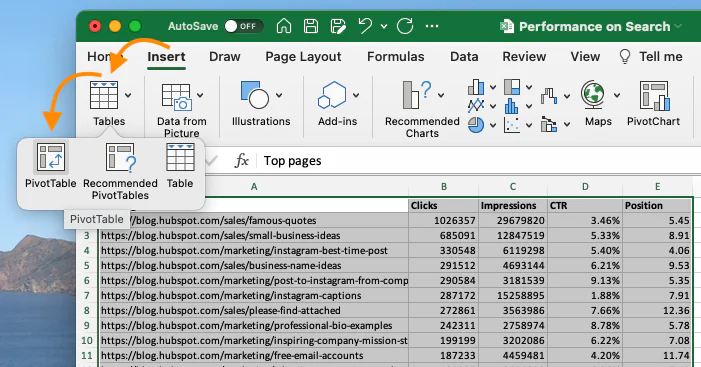
Step 3. Highlight the cells to create a custom Pivot Table
When you are done with entering data in your sheet you can easily sort things according to your taste, highlight or even summarize them in a Pivot Table. You can click at any place on your worksheet. Select your ‘Pivot Table’ and enter the list of cells you wish to include in this Pivot Table. An options box will pop up, where you can adjust the settings of cell range and confirm options like, launching a new worksheet or keep working on the existing one. If you choose to create a new worksheet you can navigate through your Excel workbook easily. Click the ‘OK’ option to confirm settings. Or you can highlight your cells and select the ‘RecommenddedPivotTables’ located towards the right side of the ‘PivotTable’ icon. Click to open this table and set your suggestions for how to manage every column and row.
Step 4. Drag and drop Your field into the “Row Labels” area
After the previous step, you have got yourself a blank Pivot Table. Your next venture is to drag and drop a field, the table is then labeled according to the names of columns in your worksheet. This is essential to identify the data according to a unique identifier like product name, blog post title, and others. You can drag and drop a field into the ‘Row Labels’ area which will allow the Pivot table to organize your data accordingly.
Step 5. Drag and drop Your field into the “Values” area
Once you have organized your data after completing the previous step, Now you are down to adding some values by dragging a field in the ‘Values’ section. By referring to the blog post example, to do this, one only has to drag the ‘Views’ field into the ‘Values’ section.
Step 6. Adjust your calculations
The total of a value is calculated by default, but it doesn’t mean you can’t change it you can easily change the sum value into a minimum, maximum, and average. You can accomplish this task by clicking on the small ‘i’ in the ‘Values’ area on Mac. Click on your desired option and select ‘OK’ to proceed with the changes. Once you are done selecting options from your Pivot Table, it will be updated accordingly. If you are working on a PC, you are required to click on the small upside-down triangle right next to your value and click on the ‘Value Field Settings’ to Land on the menu.
When you are done with categorizing your data by your fields then all you need to do is to save changes and use them in any way you please.