MS Excel is the software utilized by every business and data entry service. Setting up a budget using Excel could be overwhelming, particularly when you don’t utilize the program frequently; however, it’s easy.

 

If your budget is simple or extremely complicated, this guide will help you prepare a budget in Excel that is easily modified to meet the budgeting requirements.

 

What is a budget?

 

The term “budget” refers to a record of your earnings and the amount you can spend on your expenditures and savings. The income includes your earnings and yields through your investment portfolio.

 

How to create a budget in Excel?

 

Step 1: Open a Blank Workbook

 

The goal is to establish a Zero-based financial plan in which you record each dollar earned and spent. It’s an excellent method of keeping track of your spending because it’s precise. In all honesty, once you begin using this kind of budget, I wonder if you’ll ever need another type of budget.

 

Begin by opening Excel and selecting “Blank Workbook” or File>New>Blank Workbook. You now have a new starting point.

 

 

Step 2: Set Up Your Income Tab

 

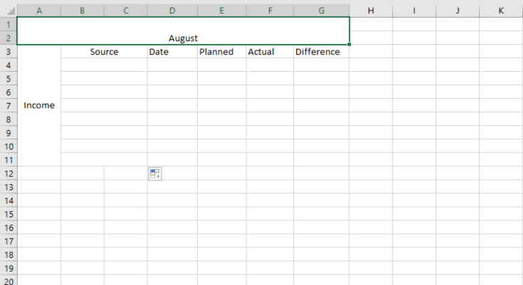
When you’ve finished creating your workbook, mark off a section of columns to be used as an introductory heading for the month. To do this, choose the first two rows of columns A-G, and then select “Merge and Center” from the workbook’s “Home” menu. This will make the entire section A1; you can name the section however you like.

 

After that, select the A3-A11 cells, select “Merge and Center,” and write the term “Income.” Suppose you want to be creative Feel free to select different colors and fonts.

 

Then, join cells C3 and B3 and label them with “Source” to represent where your income comes from in the first place – i.e., your main paycheck, your side gig, etc. You’ll also need to join every row of B&C in a separate row until row 11.

 

Label cell D3 with “Date” to help keep track of when this payment was received. A date section is optional but beneficial if your income sources change every month, and it may not be helpful when your income is predictable.

 

Next, mark section E3 with “Planned” or “Budgeted.” This represents the amount of revenue you’re anticipating earning. Section F3 will be the “Actual” column, and it’s what’s the amount that comes in. The cash deposited into the bank account will likely be more than you originally anticipated. In addition, the “Difference” column in G3 will automatically track the difference between your budgeted and actual earnings.

 

 

Step 3: Add Formulas to Automate

 

Choose all sections to help make your Excel budget look tidier. Next, select the borders tool located on the worksheet’s “Home” tab (looks like the shape of a square, divided by four) and select “All Borders.” You could shade certain areas to make it easier for you to understand.

 

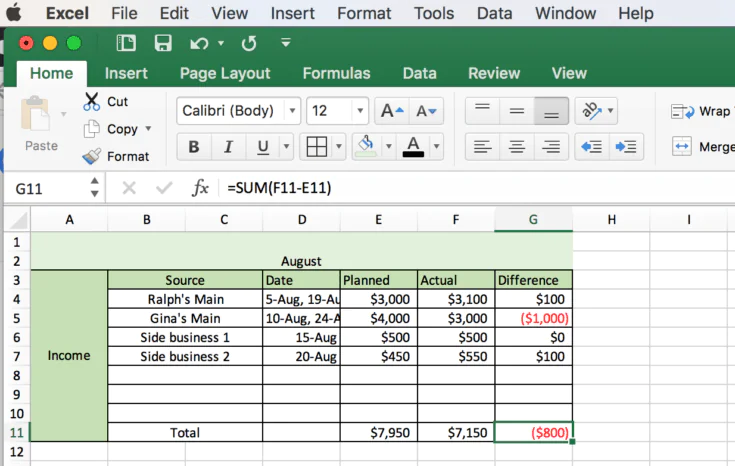
If you are satisfied with the design of the budget worksheet, it’s time to include the formulas that instantly calculate all of the expenses for you. I’ve added “Total” to the B11 cell in the following example. But you can also place it at the bottom of the list of sources of income you wish to keep track of.

 

Once you have the “Total” label, select the items from the “Planned” column and use the “AutoSum” feature to get your month’s total. Alternatively, you could choose the last line of this column and then enter this formula “=SUM(E4:E10)”. Of course, you’ll need to change those E4 and the E10 numbers with the numbers of cells you’d like to add up. Repeat the procedure to create the “Actual” and “Difference” columns.

 

To calculate automatically how much you earned between “Planned” and “Actual” income:

 

Use your equation “=SUM(F4-E4)” after each row.

 

Replace F4, E4, and E4 with the numbers corresponding to your “Actual” and “Planned” sections.

 

Repeat this process for each income row.

 

 

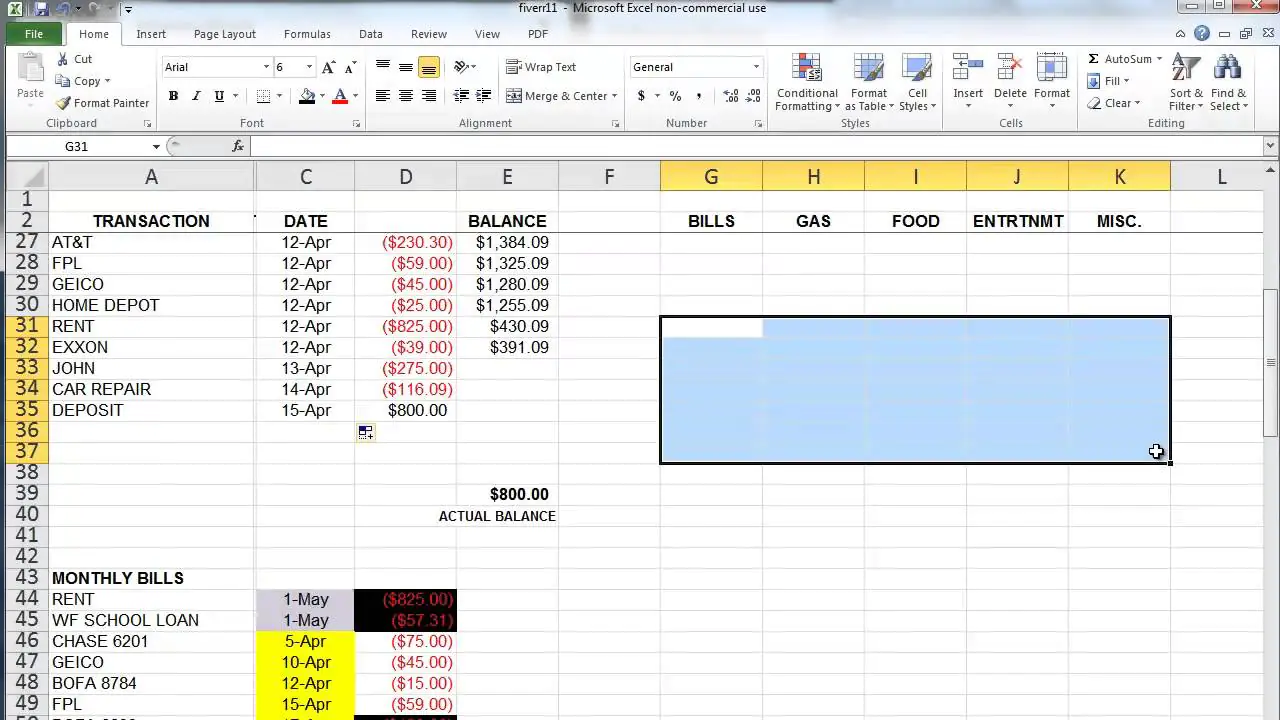
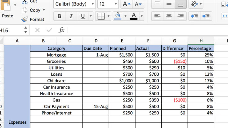
Step 4: Add Your Expenses

 

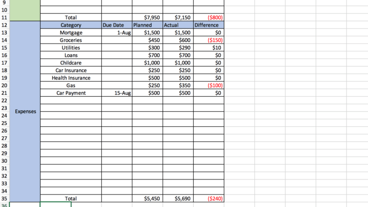
When your income and expenses are completed, it’s time to figure them out. It’s possible to complete this task on the same sheet or begin a new sheet. To ensure that expenses are on the same page, make a new section under “Income” section and customize the layout to your liking. You can then use similar column headers for columns – Due Date Actual, Planned, and Difference, similar to what you used earlier.

 

Create the formulas exactly as you did before; however, there is one major difference. In the “Difference” column, rather instead of applying an “=SUM(Actual Number-Planned Number)” formula, you’ll need to alter it. To calculate your expenses, you’ll need to apply the formula “=SUM(Planned Number-Actual Number)” to calculate the amount you’ve spent.

 

If you prefer to record the expenses separately on one page, click the + symbol on the bottom, followed by “Sheet 1.” You can then change the name of each sheet by right-clicking and choosing “Rename.”

 

When listing your expenses, you can alter the categories you prefer. It can be as specific or as broad as you’d like. The goal is to make tracking your daily expenditure simple. Some individuals might prefer to keep track of their natural gas usage, trash, and electricity separately, while others might prefer to group it under the umbrella of “utilities.” It’s your choice!

 

 

Step 5: Add More Sections

 

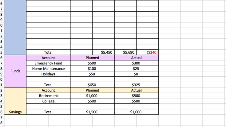
It’s time to have an enjoyable! You can add as many sheets or sections in the Excel budget as you like. I have added the “Funds” and “Savings” sections in this example. I have likely removed the “Difference” column from these sections because we don’t care about over saving. If you’d prefer to know the amount you’ve saved over what you originally planned to save, you can leave the columns in.

 

 

Step 6.0: The Final Balance

 

After completing all the sections, you’d like to track, keeping track of the running balance is essential. Fortunately, you can keep your calculator in the drawer and track it within Excel.

 

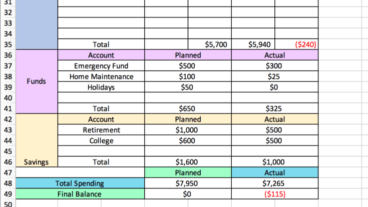
This is a breeze if you’re keeping everything on a single sheet, and you must create a second section towards the bottom. Label each row “Total Spending” and another “Final Balance.” This is a simple way to assist you in monitoring your expenditure to track your spending so you can easily compare the budgeted and actual numbers.

 

To determine the total planned budget, enter this formula “=SUM(Planned Expenses Total, Planned Funds Total, Planned Savings Total).” To determine your balance, utilize this formula “=SUM(Total Planned Spending – Total Planned Income).” The same formula applies to the balance and spending sections instead of the actual amounts.

 

Remember that for the final balance, you need to subtract the total amount you spent from the total income to arrive at an accurate figure.

 

In my fictionalized example below, the budget is exceeded by $115. Because we’ve constructed our budget with an excel spreadsheet, it’s simple to track how much the family spent and under-earned. This is the entire point of keeping track of your finances as simple as it is possible to see where every dollar is used.

 

 

Step 6.1 Add Numbers to Other Sheets

 

If you’ve created separate sheets for your expenses or savings money, you can choose which sheet you want to place the total amount on. You could either add the total to the previous sheet or create a new one solely for the balances.

 

 

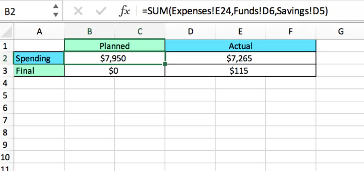
For the example above, I marked my sheets and added a total sheet at the end. The total sheet calculates the total of planned spending and the planned balance, and the sums of the actual balance and final balance.

 

To calculate the totals from different sheets, click on the cell you want the total to appear and input the formula “=SUM(SheetName!Cell, SheetName!Cell, SheetName!Cell)”. In the example, this formula would be “=SUM(Expenses!E24, Funds!D6, Savings!D5)”. Repeat this formula for your desired total and the actual amount.

 

To determine the amount you earn versus your total expenditure, click on the cell in which you would like the balance to show. Then, input the formula “=SUM(SheetName!Cell-Spending Cell)”. In the example, this is “=SUM(Income!F11-D2)”. The cell will display the negative value when you have made more money than earned.

 

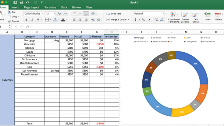
Step 7: Insert a Graph (Optional)

 

Using graphs on the spreadsheet budget is optional, but it will aid in understanding the amount you spend. To make a pie chart or bar graph to show your expenses, you’ll have to create a column that displays percentages.

 

 

As you’ll see from the example, I’ve just added a new column. To calculate the percentages automatically, this formula reads “= Total Category Cell/Actual Total Cell.” In our case, the formula will be “=F2/F24″.

 

Input this formula for every category that you want to display in percentage. For the numbers to appear as percentages instead of decimals, highlight each column and click”%” to display “%” to convert it into percentages quickly. The total percentage must equal 100 percent.

 

 

Then, highlight the category column as well as the percentage column at the same time. After both columns are highlighted, click “Insert” and choose which kind of graph you’d like to use. If you aren’t happy with the design you picked, it is possible to alter it later by right-clicking on your graph and choosing “Change Chart Type.”

 

The graph shown below is a donut graph. I love how it efficiently divides spending categories.

 

 

Thank you for taking the time to read, and best of luck!