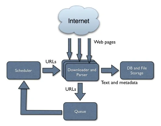
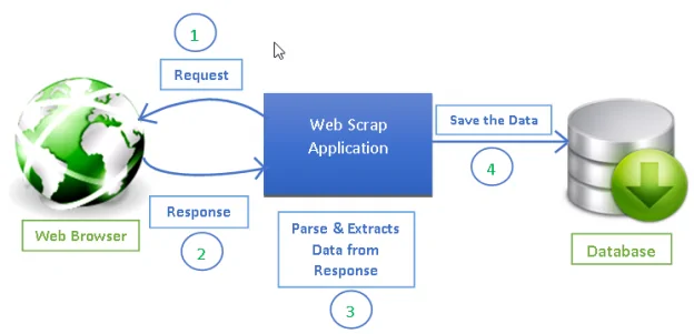
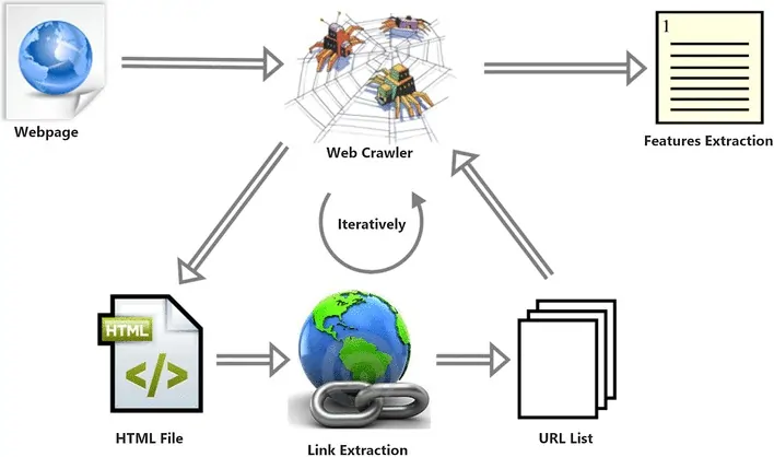
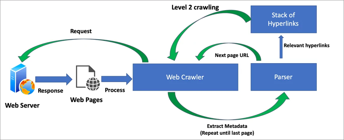
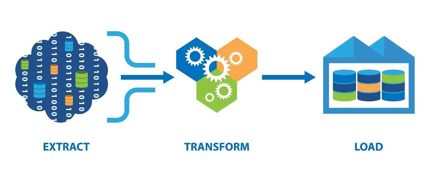
The integration of web crawlers with machine learning offers a potent approach to automate data extraction, analytics and decision-making, respectively. With the expansion of digitalization, immeasurable information is reachable online. Anyhow, navigating through these data manually takes time and proves to be ineffective. Correspondingly, web crawlers come forward as a helping hand to automate the data collection from different sites. Alike, machine learning offers intelligent analysis of target data and provides you with noteworthy insights. Essentially, web crawlers facilitate data collection, which is raw and needs to be mended, and machine learning stimulates the data collection process by processing and making predictions on the significance of gathered data. The unification of these two tools equips individuals and organizations with a streamlined workflow of data collection until its processing for taking out useful insights. This blog will present the steps to take when integrating web crawlers with machine learning to get a system that processes information and makes provision for further improvement.

 

Step 1: Setting Up Web Crawler

 

 

The primary step in integrating web crawlers with machine learning is setting up a strong web crawling component. To execute this, you need to utilize Python libraries like Scrapy, Beautiful Soup, or Selenium.

 

Scrapy is a fabulous option for more extensive projects due to its productivity and built-in highlights to oversee requests, take care of pagination, and store data. To make a basic spider in Scrapy, you’d define a class that indicates the initial URLs and the parsing logic to extract the specified information.

 

Beautiful Soup is perfect for basic tasks, particularly when you are with static pages. You can do parsing of HTML and extract data effectively by focusing on particular tags, classes, or attributes.

 

Selenium is especially valuable for dynamic websites that depend on JavaScript because it can communicate with web pages like a real client.

 

The following example involves utilizing Scrapy:

 

import scrapy

class MySpider(scrapy.Spider):

name = ‘my_spider’

start_urls = [‘http://example.com’]

def parse(self, response):

for item in response.css(‘div.item’):

yield {

‘title’: item.css(‘h2::text’).get(),

‘price’: item.css(‘span.price::text’).get(),

}

 

Once you have defined your crawler, run it to gather information, which you’ll then store in a fair format such as CSV or JSON.

 

Step 2: Processing Raw Data

 

 

After gathering data with your web crawler, the following step is to process that data. This stage is fundamental for cleaning and systematizing the raw information, ensuring it is appropriate for machine learning models. That raw data usually contains noise, irregularities, and insignificant information that can adversely affect analysis.

 

Start by removing pointless components, like HTML tags, whitespace, and special characters. For text data, you can alter everything to lowercase to preserve uniformity. Tokenization is another imperative function, to break content into individual words or expressions, which streamlines analysis.

 

After that, cope with missing or duplicate values. According to the kind of data, you can select to remove these entries or impute them with suitable values, like the mean or median. If you are operating with numerical data, normalization or scaling may be essential to confirm that all features are put up evenly to the analysis.

 

In the case of text data, consider strategies such as stemming or lemmatization to decrease words to their base forms, further improving consistency. Moreover, if your dataset incorporates categorical factors, you may ought to encode these into numerical formats utilizing one-hot encoding or label encoding.

 

Step 3: Extracting Relevant Features

 

 

Once the information is preprocessed, the following significant step is feature extraction, in which you change the tended information into an organized format appropriate for machine learning models. The quality of the features you extract can essentially impact the model’s execution.

 

In the case of text data, common procedures incorporate Term Frequency-Inverse Document Frequency (TF-IDF) and word embeddings like Word2Vec or GloVe. TF-IDF aids you in identifying the significance of words in connection to a collection of documents, successfully highlighting unique terms. For instance, you can execute TF-IDF utilizing the code as shown here:

 

from sklearn.feature_extraction.text import TfidfVectorizer

documents = [“This is the first document.”, “This document is the second document.”]

vectorizer = TfidfVectorizer()

tfidf_matrix = vectorizer.fit_transform(documents)

In word embeddings, you might utilize the Gensim library to catch semantic implications using the code:

from gensim.models import Word2Vec

sentences = [[“this”, “is”, “the”, “first”, “document”], [“this”, “is”, “the”, “second”, “document”]]

model = Word2Vec(sentences, min_count=1)

If dealing with numerical data, you can extract statistical highlights utilizing libraries like Pandas, using:

import pandas as pd

data = pd.DataFrame({‘values’: [1, 2, 3, 4, 5]})

mean_value = data[‘values’].mean()

 

If you have to deal with picture data, you can utilize strategies such as Histogram of Oriented Gradients or Convolutional Neural Networks to include extraction. Here is a basic illustration of utilizing OpenCV:

 

import cv2

image = cv2.imread(‘image.jpg’)

gray_image = cv2.cvtColor(image, cv2.COLOR_BGR2GRAY)

hog = cv2.HOGDescriptor()

features = hog.compute(gray_image)

 

Once you have the features extracted, arrange them into a structured format like a feature matrix. That matrix will function as the input for your machine learning model, empowering compelling learning and forecasts.

 

Step 4: Choosing And Preparing The Model

 

 

After extracting features from your information, the next step is to choose and prepare a machine-learning model. The selection of a model depends on the nature of your task, whether it’s classification, regression, or clustering. Each kind of issue has diverse, suitable algorithms, so understanding your information and goals is key.

 

For classification tasks, well-known algorithms include Logistic Regression, Random Forest, and Support Vector Machines. If you have to work with a regression problem, alternatives like Linear Regression or Gradient Boosting could be suitable. For more intricate tasks, particularly including image or content data, you can look into deep learning models like Convolutional Neural Networks or Recurrent Neural Networks.

 

Begin by splitting your dataset into training, validation, and test sets to assess model performance effectively. The following code is about how you can do this utilizing Scikit-learn:

 

from sklearn.model_selection import train_test_split

X_train, X_test, y_train, y_test = train_test_split(features, labels, test_size=0.2, random_state=42)

Once the data is splitting, launch and train your chosen model. For instance, if you’re employing a Random Forest classifier, the code should look like this:

from sklearn.ensemble import RandomForestClassifier

model = RandomForestClassifier()

model.fit(X_train, y_train)

 

After you have trained the model, you can assess its performance using metrics pertinent to your task.

 

Step 5: Evaluating The Model

 

 

This step contains the model assessment. This stage decides how well your model performs and whether it can successfully generalize to unseen data. Legitimate evaluation helps recognize regions for change and guarantees that the model satisfies your project’s goals.

 

Start by utilizing the validation set to regulate hyperparameters. It includes altering settings like the learning rate, the number of trees in a forest, or the profundity of a decision tree to stimulate performance. Libraries such as GridSearchCV from Scikit-learn can automate this process by observing the following command:

 

from sklearn.model_selection import GridSearchCV

param_grid = {‘n_estimators’: [50, 100, 200], ‘max_depth’: [None, 10, 20]}

grid_search = GridSearchCV(RandomForestClassifier(), param_grid, cv=5)

grid_search.fit(X_train, y_train)

best_model = grid_search.best_estimator_

 

After hyperparameters are fine-tuned, evaluate the model’s performance utilizing various metrics suitable for your task. For classification tasks, standard metrics are accuracy, precision, recall, and F1-score. Utilize the test set to urge an impartial estimate of your model’s execution:

 

from sklearn.metrics import classification_report

y_pred = best_model.predict(X_test)

print(classification_report(y_test, y_pred))

 

For regression errands, metrics like Mean Absolute Error, Mean Squared Error, or R² score are regularly utilized:

 

from sklearn.metrics import mean_squared_error

mse = mean_squared_error(y_test, y_pred)

print(“Mean Squared Error:”, mse)

 

Visualizations like confusion matrices or ROC curves can moreover give insights into model execution. In case the results are unsuitable, think of returning to previous steps to fine-tune feature extraction, alter the model, or gather more information.

 

Step 6: Model Integration And Automation

 

 

The ultimate step is integrating your prepared machine-learning model with the web crawler to form a consistent workflow for data accumulation and investigation. This integration permits for real-time handling of new data and facilitates ongoing learning and enhancements.

 

Begin by inserting your machine learning model into the web crawling pipeline. After the crawler collects information, it ought to preprocess and extract features in the same manner as during the training stage. Here’s a streamlined workflow:

 

Employ the web crawler to assemble new information.

 

Use the identical preprocessing steps you utilized during model preparing, guaranteeing uniformity.

 

Finally, Extract features with the help of the the exact strategies as earlier, preparing the data for input into the model.

 

Your integration might look like the following:

 

new_data = crawler.collect_data()

cleaned_data = preprocess(new_data)

features = extract_features(cleaned_data)

predictions = model.predict(features)

 

After that, automate this process utilizing scheduling tools such as Apache Airflow or Cron jobs to drive the crawler and model occasionally. This automation guarantees that your model persistently processes new data, giving the latest bits of knowledge.

 

Also, execute a feedback loop where model predictions can be approved against actual results. This input can educate model retraining or tuning, permitting the model to adjust and progress with time.

 

Conclusion

 

In conclusion, online platforms and websites have grown in importance as sources of unprocessed, real-time data. A web crawler facilitates methodical data browsing on web pages. It frequently scans websites to discover the content of each page so that it can be updated, indexed, and retrieved in response to user search queries. Web crawling spiders are used by various websites to update their own materials. In terms of machine learning, web crawlers are helpful in gathering data for modeling processes like training and prediction processing. When web crawlers and machine learning are combined, they add to the effectiveness of the final outcome of automatic data collection and analysis, facilitating you with a system that accommodates further improvements.