
How To Apply Any Formula In Excel? ( Excel Go-To Guide)
Digital marketers deal in information all day long, for them to analyze and categorize information in Excel spreadsheets is a hectic task. As they say, time is money, to reduce this tedious task you can make use of Excel tips and tricks all by yourself. Excel is a powerful tool that is the best-suited option for arranging numerical data and business reports. By learning these Excel hacks you can make your job simple and easy!
How to Insert Formulas in Excel?
If you are a beginner, you must be wondering what the ‘Formulas’ tab in the top navigation toolbar does? In the latest Excel version, this menu as shown below enables you to insert different Excel formulas in each cell of your spreadsheet.
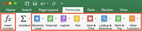
Excel formulas also known as ‘functions’ are used to highlight a cell in which you wish to run the formula, followed by the left icon ‘Insert Function’ to get access to other popular formulas and their functions. Let us discuss these formulas one by one:
1. SUM
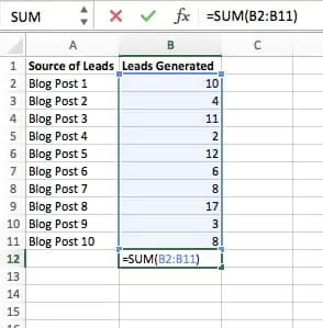
All kinds of Excel formulas start with an ‘=’ symbol which is followed by a text tag that includes the formula that you wish to insert. SUM formula is the basic Excel formula used to add two or more values in cells. To perform this formula, at first, you need to enter values that you want to add together using the format: =SUM (value 1, Value 2, … etc). Value of this formula is equal to a certain cell in your spreadsheet.
For example, let us consider the SUM of the values B2 and B11. For this, we will have to enter =SUM(B2, B11), the cell will result in a total of the numbers filled in these two cells. Although if there are no numbers in these two cells, the result will be 0.
2. IF
The IF formula is represented as =IF(logical_test, value_if_true, value_if_false). This formula allows you to enter a value if there is something true or false in your spreadsheet. For instance, =IF(D2=”Gryffindor”,”10″,”0″) will result in 10 points to cell D2 if it has the word ‘Gryffindor’. Therefore if you wish to add 10 points to everyone belonging to Gryffindor’s house then you can directly add these points by using this formula and skip the manual part.
Value_if_True: If in case the value is true then the number 10 is awarded to the students. You can use quotation marks if you want the result to be displayed in text and not numerics.
Value_if_False: If the value is false then the student does not get any bonus points – we will get “0” in place of 10 points.
3. Percentage
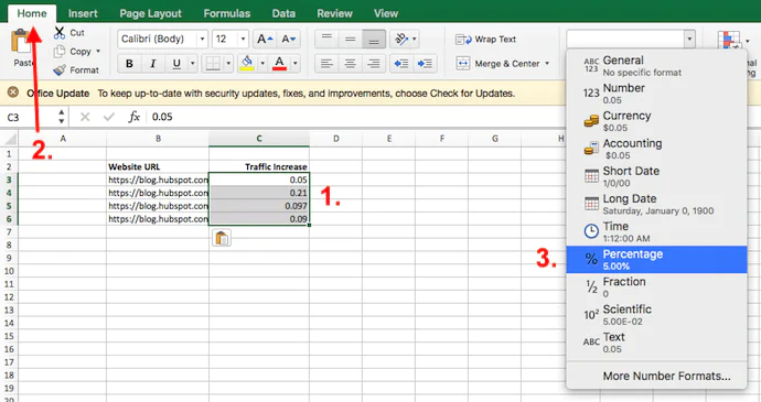
To perform the percentage formula in an Excel spreadsheet you need to enter cells that you desire to find the percentage for in the formula format, =A1/B1. You can easily convert the decimal value to a percentage by following a few simple steps:
Highlight the cells that you want to multiple.
Click on the Home tab and select the ‘Percentage’ option from the menu dropbox.
Select the relevant tab and change the menu next to conditional formatting which says ‘General’ as the default setting.
Select ‘Percentage’ from the list that appears on the screen. This will result in a percentage of all the highlighted cells. As shown below;
4. Subtraction
To perform the subtraction formula in an Excel spreadsheet, you must enter data into the cells that you want to subtract and perform the action by applying the format =SUM(A1, -B1). This will result in the subtracted value of the two or more cells. Using the SUM formula and adding a negative sign before the cell you want to subtract is all that you require to act successfully. For example, if B1 is 6 and A1 is 10 then by applying this formula you would get 10 + -6, the value of 4.
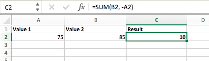
Using the =SUM formula. To subtract one value from another, at first enter data into the respective cells and apply format =SUM(A1, -B1), the only thing included in this format is a negative sign which is denoted with a hyphen. You will have to press enter to find out the difference between the two cells.
Using the format, =A1-B1. To subtract more than two values you are only required to add an equal sign before the first cell, a hyphen, and other values that you wish to subtract. Press ‘Enter’ to get instant results.
5. Multiplication
This Excel formula is used to perform straightforward multiplication of cells in the format, =A1*B1. This format includes an asterisk to command the multiplication of the selected cells. For example, if A1 is 10 and B1 is 6 applying the format =A1*B1 would result in the value of 60.
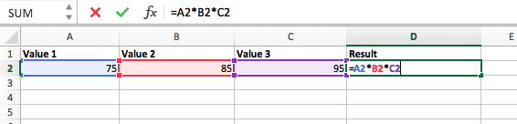
To multiply two or more cells in an Excel spreadsheet you will have to highlight an empty cell. All the values will be multiplied together in the format, =A1*B1*C1… etc. The asterisk commands the multiplication of values included in the cells and when you press ‘Enter’ you get the desired product.
Excel Keyboard Shortcuts
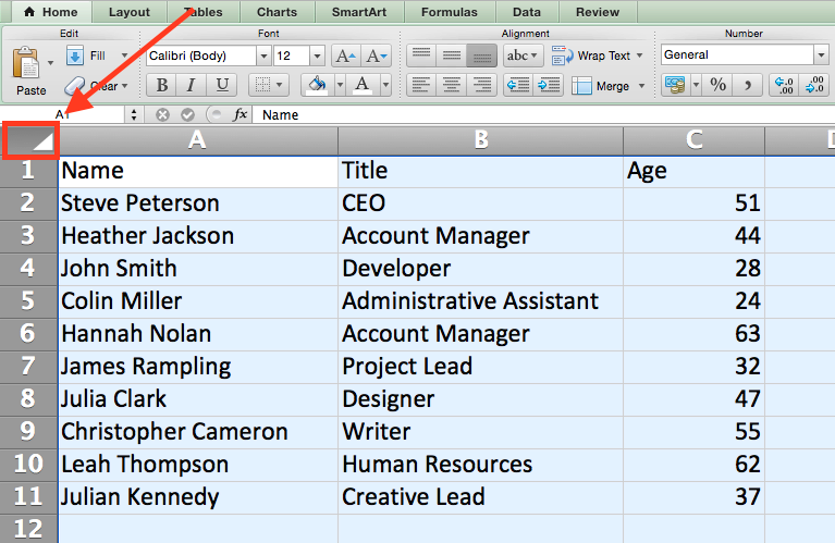
Quick Selection of Rows, Columns, or Whole Spreadsheet
Perhaps you are short on time, well who isn’t in this fast-paced world. You can highlight the whole spreadsheet in just one click. All you need is to click on the tab at the very top left corner of the spreadsheet and select every cell at once.
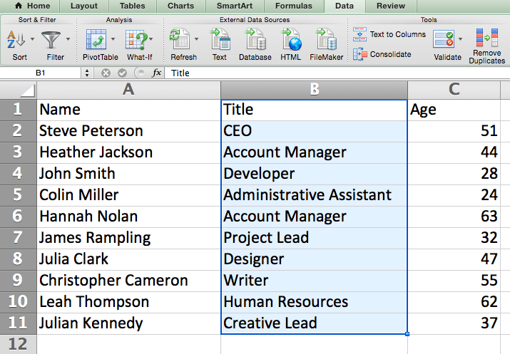
If you wish to select everything in a particular row or column then you must be aware of these shortcuts:
For PC:
Select Column = Control + Shift + Down/Up
Select Row = Control + Shift + Right/Left
For Mac:
Select Column = Command + Shift + Down/Up
Select Row = Command + Shift + Right/Left
Both these shortcuts are beneficial if you are working on larger datasets and need to select a specific part of them.
2. Quick Performance of Open, Close, or Create a Workbook Actions
You can easily open, close, or create a workbook by knowing keyboard shortcuts. It will enable you to complete all of the above-mentioned actions in less than one minute.
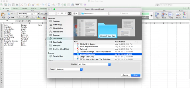
For Mac:
Open = Command + O
Close = Command + W
Create New = Command + N
For PC:
Open = Control + O
Close = Control + F4
Create New = Control + N
3. Easy Formatting of Numbers into Currency
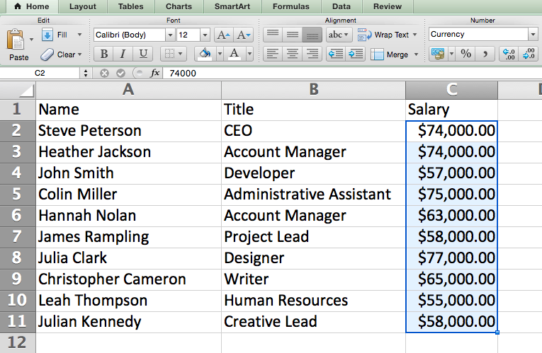
You can easily convert raw data into currency or any figure like salary, sales tickets, marketing budgets for an event, and more. For this purpose, you need to highlight the respective cells and select Control+Shift+$.
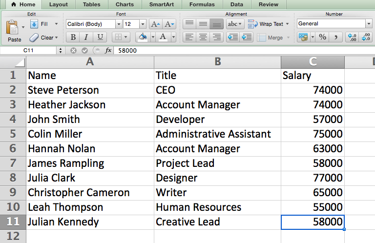
Numbers will be translated automatically into currency consisting of commas, dollar signs, and decimal points.
This shortcut is also applicable to percentages ‘%’ as well. In percentage conversion, if you want to convert numerical values as percentage figures then you will replace the ‘$’ sign with ‘%.’
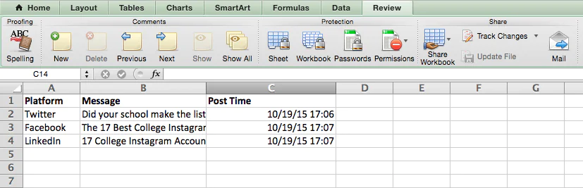
4. Insertion of Date and Time into any Cell
You might want to add the current date and time while checking social media posts or your business to-do lists. You can easily enter the time and date stamp into your spreadsheet by selecting the specific cell to which information must be added. The formatting procedure for data and time is given below:
Insert current time = Control + Shift + ; (semi-colon)
Insert current date = Control + ; (semi-colon)
Insert current date and time = Control + ; (semi-colon), SPACE, and then Control + Shift +; (semi-colon).
Some Other Excel Tricks
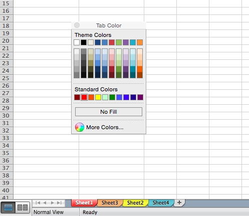
1. Customize Tab Color
If you are working on various sheets in one workbook, then you can make things recognizable by color coding the tabs. For instance, you can label the reports of previous months with red color and the report of this month with orange color. You can simply click on the ‘Tab Color’ option and choose a certain color you want as a tab theme or you can customize one for yourself based on your needs.
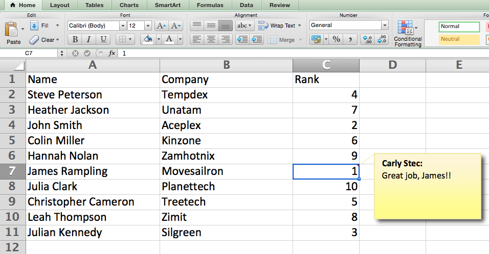
2. Add New Comments
Whenever you wish to make an addition of a comment or a note to a certain cell within the spreadsheet, rather than changing the whole spreadsheet you can simply right-click on the specific cell and then enter the ‘Insert Comment’ option. Next, you can type in your comment directly in the text box and click ‘Enter’ to save changes. Cells that include comments display a red triangle in the corner. You can view your comment by sliding over the red triangle.
3. Copy and Duplicate Formatting
When you spend a lot of your time formatting the spreadsheet according to project demands then you might as well agree that it is an uninteresting task that gets tedious with every passing minute. For this very reason, it has become important to learn a few tips and tricks to not repeat every process right from the start. By using the ‘Excel Format Painter now you can easily copy the formatting of one sheet and paste it to another.
It is rather a replication process that enables you to copy the area that you wish to replicate and then click on the ‘Format Painter’ option to select the ‘Paintbrush’ icon by accessing the dashboard. Using the paintbrush pointer, you can successfully select the desired cell, text, or the entire spreadsheet to your liking and apply the formatting as referenced below:
4. Identify Duplicate Values
In many circumstances handling duplicate values can be challenging for example, in SEO managing duplicate content might prove troublesome when it is not corrected in time. You must be aware of such situations as problems can surface at any time. It is easy to manage duplicate values by following certain steps closely. Right, click on the ‘Conditional Formatting’ option and from there select ‘Highlight Cell Rules > Duplicate Values’.
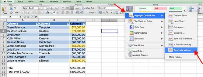
Using this pop-up you can efficiently format your desired rule and specify a duplicate value in the spreadsheet.
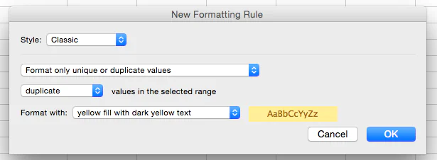
In the example given above, we are trying to identify duplicate values within this selected area and format the duplicate cells in yellow color. In the marketing business, the use of Excel is extensive and inevitable. All the aforementioned formulas, tricks, and tips can help make Excel easy and simple for your daily business ventures.