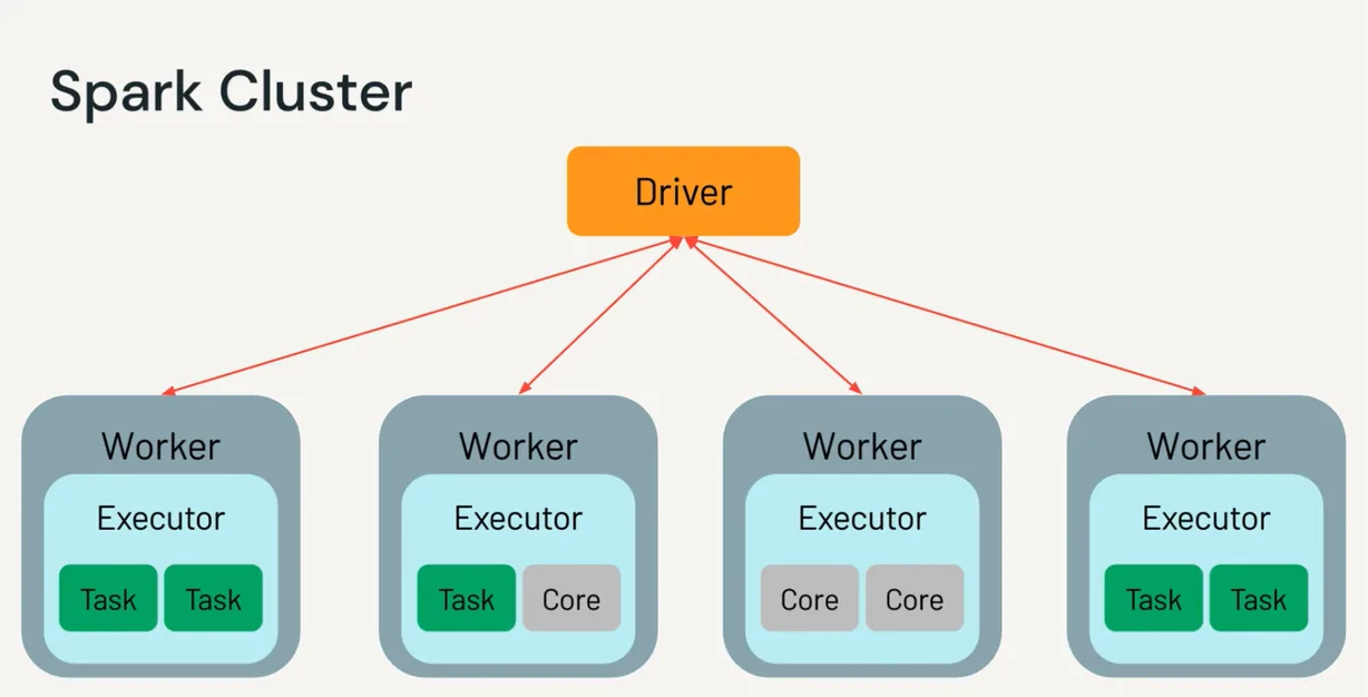
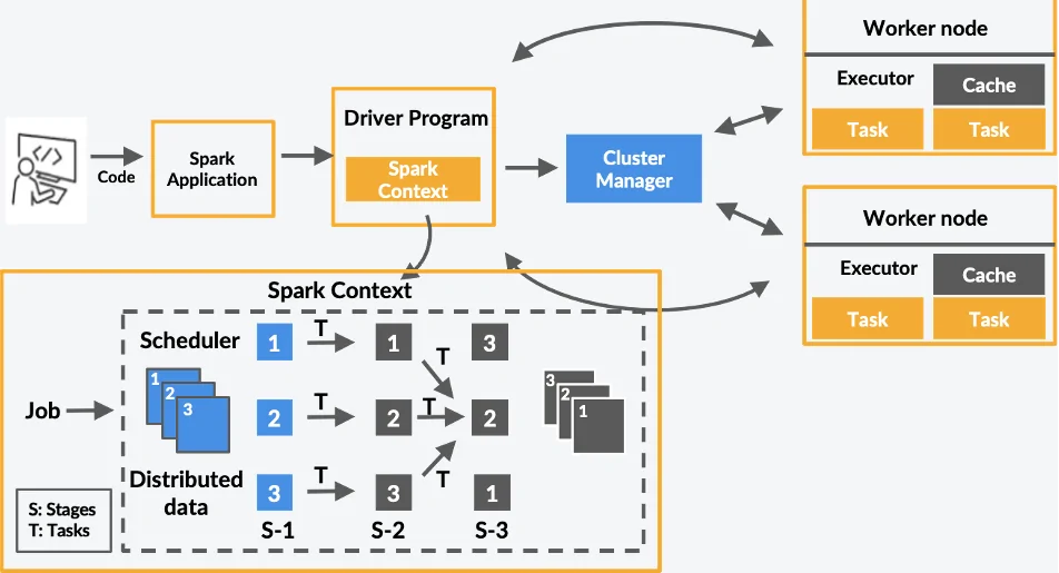
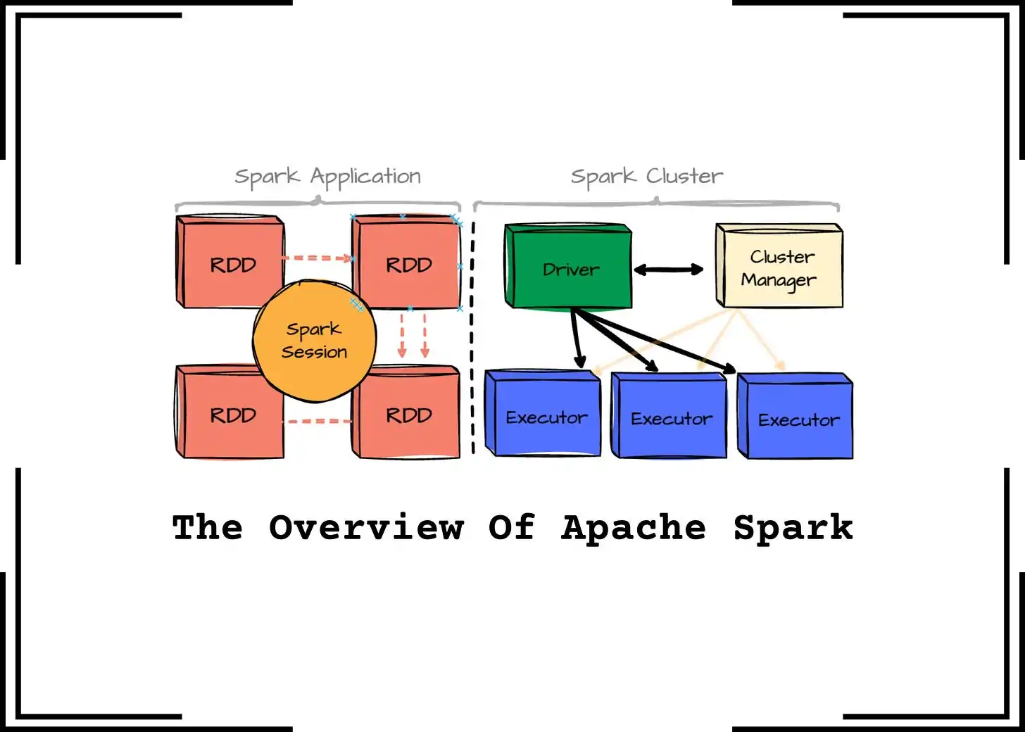
Large datasets are processed using a variety of measures and techniques to create formats that are appropriate for consumption. The objective is to extract relevant data that can be used to support current technologies or be employed in decision-making processes. Data collection, filtering, sorting, and analysis are frequently the main processing steps to handle big datas. Data scientists and engineers use a combination of data processing tools and methods to successfully navigate these phases, guaranteeing that the final product is accurate and worthwhile. Spark is one such tool that presents a comprehensive, unified framework to deal with big data processing requirements with an assortment of data sets that are manifold in nature as well as the sources. Here, data sets stand for both structured and unstructured data, and also various sources, including social media pages, sensors, and logs, all chipping into the complexity and abundance of the data. The primary components of Apache Spark’s architecture include Data Storage, API and Management Framework. All these components, along with various others, work together to ensure the effectiveness of Spark’s distributed data processing. The following steps of this blog will demonstrate how Apache Spark can handle large data sets quickly and efficiently.

 

Step 1: Data Ingestion In Apache Spark

 

 

Data ingestion in Apache Spark is the method of loading huge volumes of information from distinctive capacity frameworks into Spark for examination. The distributed nature of Spark makes it exceedingly appropriate for dealing with enormous datasets by reading the information in parallel across nodes, lessening bottlenecks and racing up loading times. Typical sources incorporate HDFS, Amazon S3, databases, and also local files, and Spark’s adaptability permits ingestion of organized, semi-structured, and unstructured information.

 

The selection of data format from options such as CSV, JSON, Parquet, or ORC can influence the way data can be processed productively, with columnar formats, like Parquet, presenting performance benefits for huge, complex datasets.

 

During the ingestion process, setting choices, including headers, delimiters, and schema inference, guarantees that Spark translates the data accurately. For example, for a CSV file with headers, designing options avoids issues in column arrangement and data type identification. In the following section is a code illustration for ingesting a CSV file utilizing Spark’s DataFrame API:

 

from pyspark.sql import SparkSession

# Initialize Spark session

spark = SparkSession.builder.appName(“DataIngestionExample”).getOrCreate()

# Load data from a CSV file

df = spark.read.format(“csv”) \

.option(“header”, “true”) \

.option(“inferSchema”, “true”) \

.load(“hdfs://path/to/data.csv”)

# Display the first few rows

df.show()

 

That code will make a DataFrame from the ingested information, empowering further modification and analysis over Spark’s nodes.

 

Step 2: Cleaning And Planning Loaded Data

 

 

After the data is loaded, the following step is to clean and plan it, making sure it is appropriate for analysis. Data cleaning in Spark includes dealing with missing values, disposing of duplicates, and adjusting inconsistencies within the data set. The DataFrame API  of Spark’ gives straightforward functions for these errands, such as dropna() to expel rows with invalid values and dropDuplicates() to filter out duplicate sections.

 

During preparation, you can include new columns, apply transformations, or cast data sorts to fulfill analysis prerequisites. For example, employing withColumn() permits you to form derived columns or adjust existing ones. It is, moreover, typical to apply filtering with filter() to hold only pertinent information.

 

Below is an illustration of code for data cleaning and preparing:

 

# Drop rows with any missing values

df_cleaned = df.dropna()

# Remove duplicate rows

df_cleaned = df_cleaned.dropDuplicates()

# Add a new column with transformed data

df_cleaned = df_cleaned.withColumn(“sales_tax”, df_cleaned[“sales”] * 0.07)

# Filter for relevant data

df_cleaned = df_cleaned.filter(df_cleaned[“status”] == “active”)

 

These actions ensure your data is watchful for efficient processing within the following phases.

 

Step 3: Transforming Prepared Data

 

 

Data transformation is vital in shaping information to conform to analysis necessities. In Spark, transformations include using operations such as filtering, choosing particular columns, and modifying data to acquire profitable insights. the DataFrame API of Spark presents functions like filter(), select(), groupBy(), and join() to attain effective data transformations. These operations work over Spark’s distributed nodes, permitting expansive datasets to be handled rapidly.

 

Filtering, for instance, can decrease data size by extracting insignificant records, while preferring particular columns can help emphasize pertinent data traits. More complex changes, such as grouping and joining different DataFrames, empower thorough data investigation by incorporating affiliated datasets and performing aggregate calculations.

 

The following example code illustrates some typically performed transformations:

 

# Filter data based on conditions

df_transformed = df_cleaned.filter(df_cleaned[“age”] > 18)

# Select specific columns for analysis

df_transformed = df_transformed.select(“name”, “age”, “city”)

# Group data and calculate the average age by city

df_grouped = df_transformed.groupBy(“city”).avg(“age”)

# Join with another DataFrame on a common column

df_final = df_grouped.join(other_df, df_grouped[“city”] == other_df[“city_id”], “inner”)

 

The above transformations will tailor the data, stimulating important insights and preparing data for computations in consequent stages.

 

Step 4: Deriving Insights From Data

 

 

This step involves aggregation and computation, which is about summarizing, calculating, and deriving insights from the data. In Spark, it is usually accomplished utilizing operations such as groupBy(), agg(), and join(), permitting high-level calculations over expansive datasets. Aggregations help consolidate information, like summing sales figures by area, discovering average values, or counting occurrences inside categories. Computation also incorporates any factual or numerical operations mandated for analysis.

 

The distributed processing aspect of Spark proficiently addresses these tasks by partitioning them across nodes. Aggregating and computing on expansive data sets can be favorably parallelized, making it appropriate for use cases that mandate speedy outcomes over massive information volumes.

 

Below is a code illustration that represents typical aggregation and computation processes:

 

# Group data by category and calculate total sales per category

df_aggregated = df_transformed.groupBy(“category”).agg({“sales”: “sum”})

# Calculate average sales and maximum profit within each region

df_stats = df_transformed.groupBy(“region”) \

.agg({“sales”: “avg”, “profit”: “max”})

# Perform additional computations, such as total transactions per customer

df_customer_transactions = df_transformed.groupBy(“customer_id”).count()

 

This step compacts information into significant outlines, offering insights that drive decisions in further investigation and reporting phases.

Step 5: Optimizing Dataframe Operations

 

 

Optimization and tuning are fundamental to enhancing Spark’s performance, particularly with huge datasets. In this stage, you will modify Spark’s setups and optimize DataFrame operations to lower handling time and resource utilization. Essential moves incorporate partitioning, caching, and configuring resources such as memory and CPU allocation. Appropriate partitioning of information guarantees that tasks are offset over Spark nodes, preventing processing delays caused by skewed data distribution. Caching is another strategy, especially valuable when data is reused, because it stores DataFrames in memory, eliminating the got to recompute data.

 

Modifying Spark’s implementation settings like spark.sql.shuffle.partitions or spark.executor.memory can also upgrade productivity by allocating resources successfully.

 

The following example will present standard optimization strategies:

 

# Repartition data for better load distribution

df_optimized = df_final.repartition(10)

# Cache data if it will be reused multiple times

df_optimized.cache()

# Configure Spark settings for optimized performance

spark.conf.set(“spark.sql.shuffle.partitions”, “50”)

spark.conf.set(“spark.executor.memory”, “4g”)

 

The above optimizations guarantee that Spark utilizes cluster resources proficiently, making large-scale data handling speedier and more reliable.

 

Step 6: Saving The Processed Data

 

 

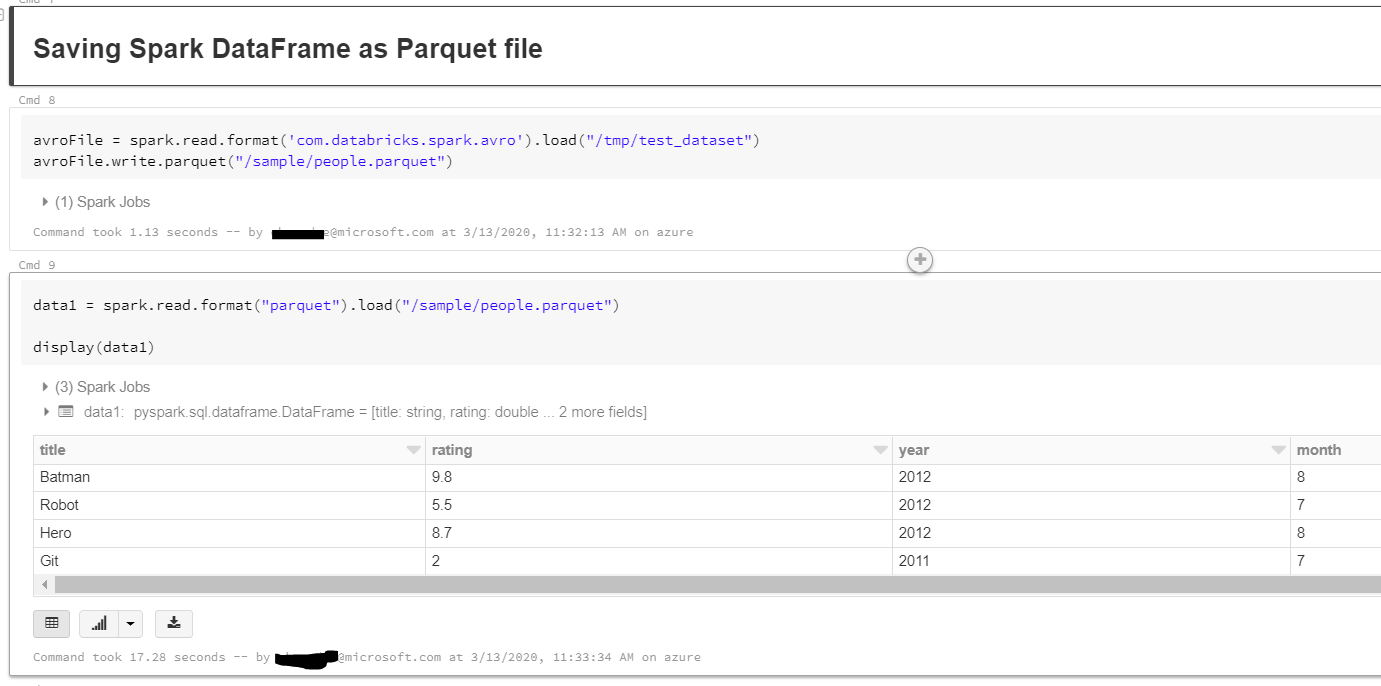
After the data is handled and optimized, the ultimate step is to output and store the outcomes. Spark permits you to save the handled data in different formats, like CSV, Parquet, JSON, or even in databases. The selection of the format relies on the use case and future processing prerequisites. For instance, columnar formats such as Parquet offer efficient storage and more rapid reads, while CSV may be reasonable for compatibility with other tools.

 

In this stage, you define the output location like HDFS, S3, or local file framework and indicate the file format and alternatives. You can also segment the output information to optimize capacity and retrieval. Furthermore, Spark gives the choice to overwrite existing information or add new results.

 

The following is code example to preserve the data:

 

# Save the processed data as a Parquet file

df_final.write.format(“parquet”).mode(“overwrite”).save(“path/to/output_data”)

# Save data as CSV with header

df_final.write.option(“header”, “true”).csv(“path/to/output_csv”)

# Save data to a database (e.g., MySQL)

df_final.write.format(“jdbc”).option(“url”, “jdbc:mysql://localhost:3306/mydb”) \

.option(“dbtable”, “processed_data”).save()

 

This action guarantees that the processed information is stored in a organized format, all set for use in downstream applications, reporting, or additional examination.

Conclusion

 

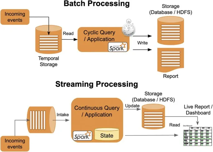
To sum up, Apache Spark is a widely used big data distributed processing framework that can be deployed in a number of ways. Its native bindings for the Java, Scala, Python, and R programming languages, and support to SQL, streaming data, machine learning, and graph processing make it inevitable for organizations including Banks, telecommunications companies, gaming companies, governments, and all of the major tech giants. They use Apache Spark as many of its features facilitate quickly completing processing tasks on very large data sets and distributing data processing tasks across multiple computers, either independently or in conjunction with other distributed computing tools.