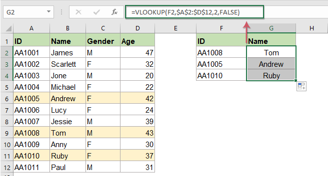
Excel’s VLOOKUP function is an effective tool used in a variety of businesses to obtain data from a table by utilizing a lookup value. It returns a corresponding value in the same row with a given column after searching for a value in the first column of a range like a table or array. Given that the “V” in VLOOKUP stands for “Vertical,” it searches a table vertically or downward. In order to locate a match, VLOOKUP searches along a table’s first column. It obtains information from the designated column of the same row after finding that match. For instance, if you want to know the price of a product, Excel’s VLOOKUP function searches the product list, locates the one you want, and then provides the price from the relevant column. VLOOKUP is a really valuable tool, and learning how to use it is easier than you may expect. All you need to do is grasp the fundamentals of functions and adhere to a methodical process like the one mentioned below:

 

Step 1: Sorting The Lookup Column

 

 

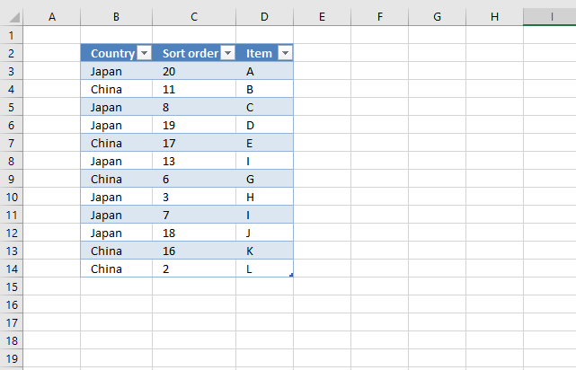
The first phase of the process is sorting the lookup column, which can significantly improve the execution of VLOOKUP, particularly when you are dealing with huge datasets. After the 4th argument of VLOOKUP is specified to True, Excel assumes the data is sorted in ascending order and executes a binary search, which is much speedier than exploring each row sequentially. This strategy minimizes the number of comparisons, making information retrieval nearly moment in expansive spreadsheets.

 

If the column is unsorted and the approximate match is empowered, VLOOKUP might yield inaccurate outcomes.

 

To perform sorting of the column, select the lookup column, head to the Data tab, then press Sort A to Z. Make sure that the sorting accommodates the dataset’s structure to preserve data integrity. In case too many upgrades are made to the dataset, look into automating the sorting process utilizing Excel’s built-in highlights, such as Power Query or VBA Macros.

 

For correct matches, sorting does not improve speed essentially, but it still makes a difference in keeping up an assembling dataset. If sorting the initial dataset isn’t a choice, think about making a sorted helper column utilizing Excel formulas or Power Query, and after that, reference it in VLOOKUP. That minor alteration can greatly improve lookup speed, decreasing lag in large Excel files.

 

Step 2: Utilizing The Approximate Match

 

 

Utilizing the approximate match choice in VLOOKUP speeds up searches, particularly in expansive datasets. Once you set the Excel to Trueit, it will run a binary search, which is incredibly speedier than checking each row individually. That strategy will minimize the number of comparisons, making it perfect for datasets with thousands of entries. In any case, to utilize this proficiently, the lookup column should be sorted in ascending order, guaranteeing that Excel can quit searching once it locates the closest match.

 

The surmised match is especially valuable when performing with numeric ranges, like tax brackets, commission structures, or grading systems. For instance, if you have a table containing sales ranges and compare bonuses, utilizing True in VLOOKUP will let Excel rapidly discover where a value falls inside the range.

 

To execute this function, you will structure your equation this way:

 

=VLOOKUP(A2, B2:D1000, 2, True)

 

On the off chance that the dataset demands exact matches like product codes or employee IDs, the approximate match must not be utilized because it may yield unexpected results. In any case, when dealing with expansive sorted datasets where an exact match isn’t needed, empowering True will essentially boost Excel’s execution and diminish processing duration.

 

Step 3: Limiting The VLOOKUP Range

 

 

Limiting the VLOOKUP range to exclusively the fundamental rows and columns enhances speed and minimizes processing time. Numerous users select entire columns like B:D or pointlessly expansive ranges like B2:D100000, pushing Excel to check intemperate information, driving slow execution. Rather, define the smallest possible range that covers the required data.

 

For instance, in case your table has 3 columns and 500 rows, rather than utilizing:

 

=VLOOKUP(A2, B:D, 2, False)

You can utilize:

=VLOOKUP(A2, B2:D500, 2, False)

 

It will define the lookup operation, averting Excel from looking at pointless, empty or unessential cells. Furthermore, converting huge datasets into Excel Tables with Ctrl + T makes range administration dynamic, automatically altering as data develops. You can also employ dynamic named ranges with equations such as Offset or Index. For instance, specify a named range utilizing the equation:

 

=OFFSET(B2,0,0,COUNTA(B:B),3)

 

That approach can adjust the range according to the real data, guaranteeing proficient lookups.

 

Step 4: Including A Helper Column

 

 

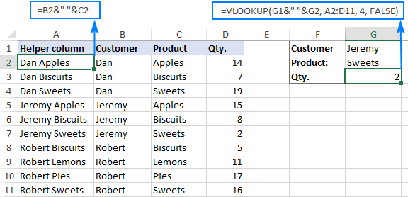
The addition of a helper column will provide a swift VLOOKUP to handle huge amounts of data. It condenses information into a single searchable key, thus relieving users from dealing with multiple columns.

 

For instance, if looking up data per first and final names, rather than utilizing VLOOKUP independently on two columns, you can make a helper column that connects them:

 

=A2 & ” ” & B2

 

After that, you need to reference this helper column in VLOOKUP:

 

=VLOOKUP(D2, E2:G5000, 2, False)

 

Another method to optimize execution is by utilizing binary search with an approximate match on a helper column that sorts values consistently. That strategy will decrease lookup time from linear (O(n)) to logarithmic (O(log n)) complexity, essentially upgrading the rate in huge datasets.

 

Step 5: Improving Speed And Adaptability

 

 

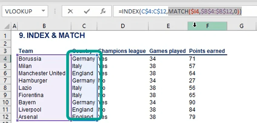
The replacement of VLOOKUP with the INDEX-MATCH combination improves speed and adaptability, particularly in the case of expansive datasets. In contrast to VLOOKUP, which searches from left to right and checks whole ranges, INDEX-MATCH specifically retrieves information by finding the precise row number foremost, making it incredibly quicker.

 

The standard INDEX-MATCH formula is as follows:

 

=INDEX(C2:C5000, MATCH(A2, B2:B5000, 0))

 

That formula is more proficient because its MATCH component finds the row position first, and the INDEX retrieves the value immediately.

 

Moreover, in contrast to VLOOKUP, which needs the lookup column to be the leftmost, INDEX-MATCH can search in multiple directions.

 

Also, the VLOOKUP recalculates the complete range, while INDEX-MATCH confines only the specified column.

 

For even more prominent speed, utilize an approximate match like 1 or -1 rather than a correct match like zero while performing with sorted data. Look into the following formula:

 

=INDEX(C2:C5000, MATCH(A2, B2:B5000, 1))

 

It will empower binary search, altogether lessening lookup time from O(n) to O(log n). Substituting VLOOKUP with INDEX-MATCH could be a basic, however capable, way to facilitate Excel execution.

 

Step 6: Converting The Formulas

 

 

Once you have conducted VLOOKUP for data retrieval, making the formulas active can slow down Excel, particularly in the case of expansive datasets. Transforming VLOOKUP results into static values diminishes processing time and enhances comprehensive execution. It is because Excel recalculates formulas each time the worksheet upgrades, even if the lookup values stay unaltered.

 

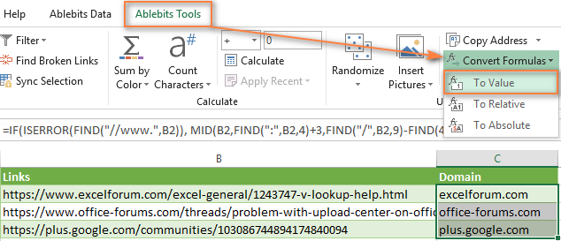
To change over formulas into values, look into the following phases:

 

Choose the cells that contain VLOOKUP formulas.

 

Utilize the Ctrl + C keys to copy the formulas.

 

Finally, right-click and select Paste Special, then Values or tap on Ctrl + Alt + V, next V.

 

It will substitute the formulas with their recent outcomes, avoiding unneeded recalculations. In case upgrades are required, keep the original lookup formulas in a partitioned worksheet and refresh them as essential before pasting them as values.

 

For superior effectiveness, utilize Power Query to drag and transform data, lessening the requirement for manual lookups. Another option is utilizing PivotTables, which gives an organized way to retrieve values without running formulas over and over.

 

By switching lookup results to values, Excel will operate quicker, consume slightly more memory, and avoid execution lags driven by excessive formula calculations in huge spreadsheets.

 

Conclusion

 

To sum up, Excel’s VLOOKUP gives individuals flexibility based on their needs by allowing for precise and approximate matches. Finding relevant information without manually searching through rows is made easier by VLOOKUP, which speeds up data retrieval from enormous databases. Users can use it to merge data from various tables. Particularly when working with large datasets, automating the lookup procedure saves time. Without repeatedly entering data by hand, users can rapidly refer to and examine it. In addition, compared to manual data entering and searching, VLOOKUP lowers the possibility of human oversights, resulting in more accurate data analysis.